Advanced Conditional formatting

Common Steps

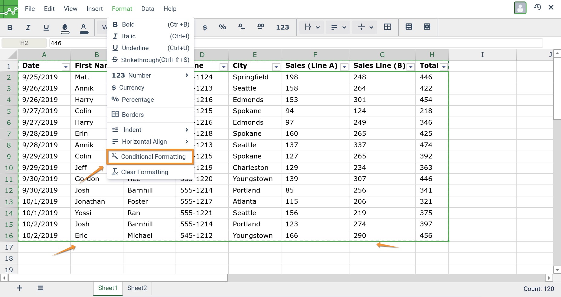
Open a confluence page and create a new Excellentable or edit an existing Excellentable.
Select the cells you want to apply format rules to.
Click Format and then Conditional formatting. A toolbar will open to the right.

Highlight unique or non-unique cells

Create a rule by choosing the condition and the style if required.
In this example we want to find all the names that show up only once in the records (Select the Cells B2:B16).
In "When" select value "this formula is true", and in the formula field "=$H2>409" to select the condition. Select the background color (light green) and select the font color (dark green). Click "Add Rule".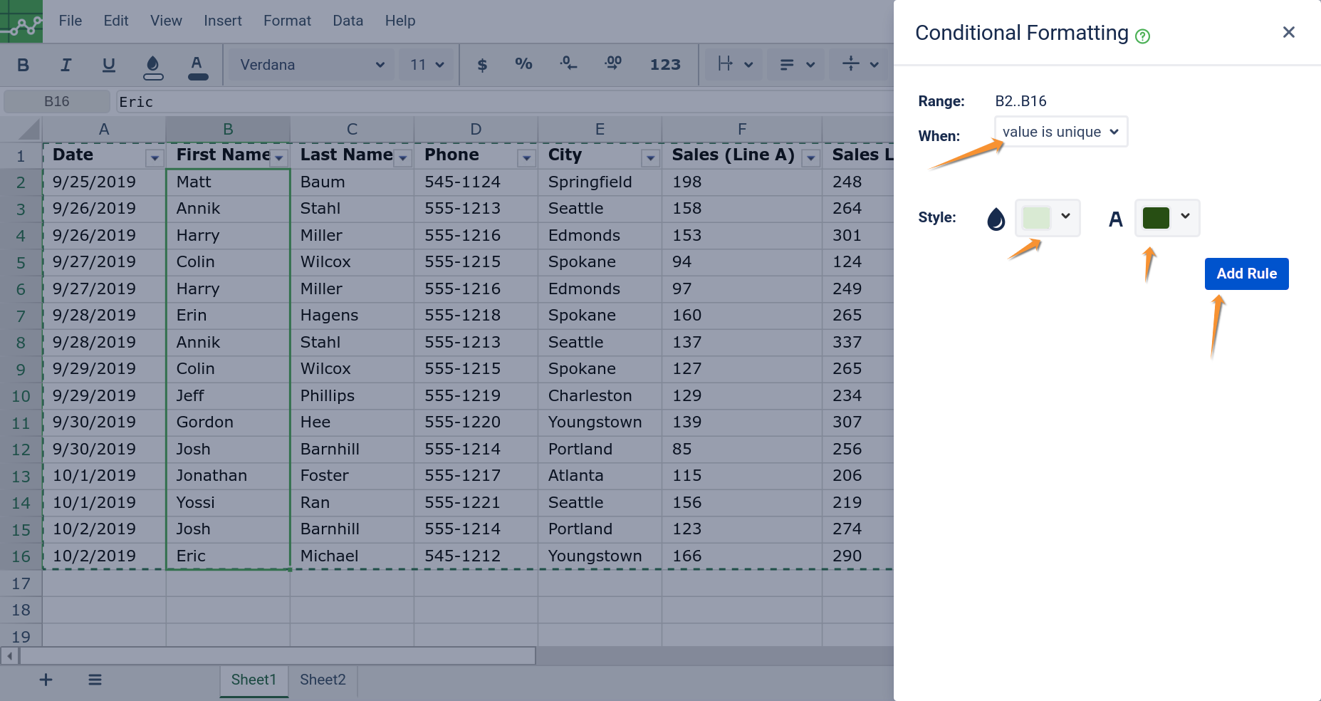
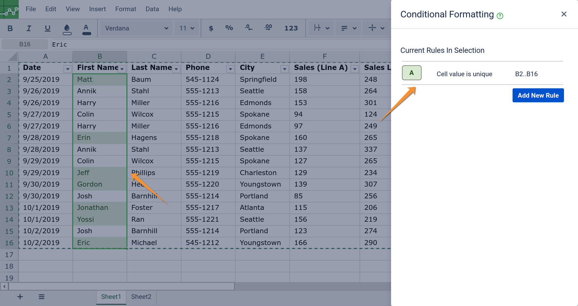
Add another Rule (If required) If multiple rules are required, you can stack rules together.
Exit after you have applied all the required rules. Your Excellentable should show the rules in the Conditional formatting now.

Create a rule by choosing the condition and the font if required
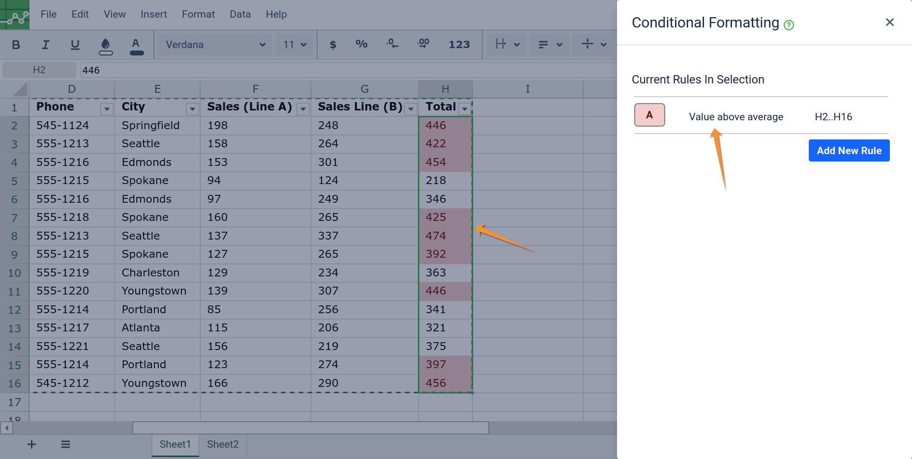
In this example we want to find all the total sales values that are above average (Select the Cells H2:H16).
In "When" select value "by average cell is", and in the in the dropdown field above average. Select the background color (light red) and select the font color (dark red). Click "Add Rule".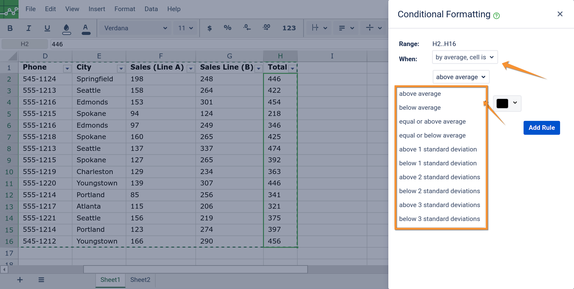
Add another Rule (If required) If multiple rules are required, you can stack rules together.
Exit after you have applied all the required rules. Your Excellentable should show the rules in the Conditional formatting now.

Data bars will fill the background of cells based on the values, like a bar graph.
Create a rule by choosing the condition and the font if required.
In this example we want to highlight the sales (Line B) as a bar based on the values.
In "When" select value "values in data bar rule", In "Min" dropdown select "Automin" and in the "Max" dropdown select "Automax". Select the background color (light green). Click "Add Rule".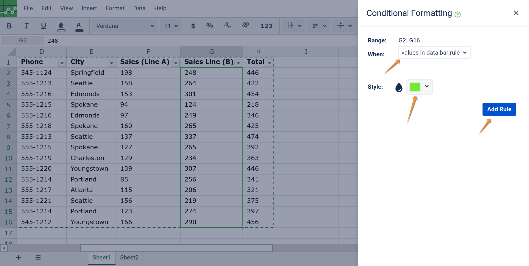
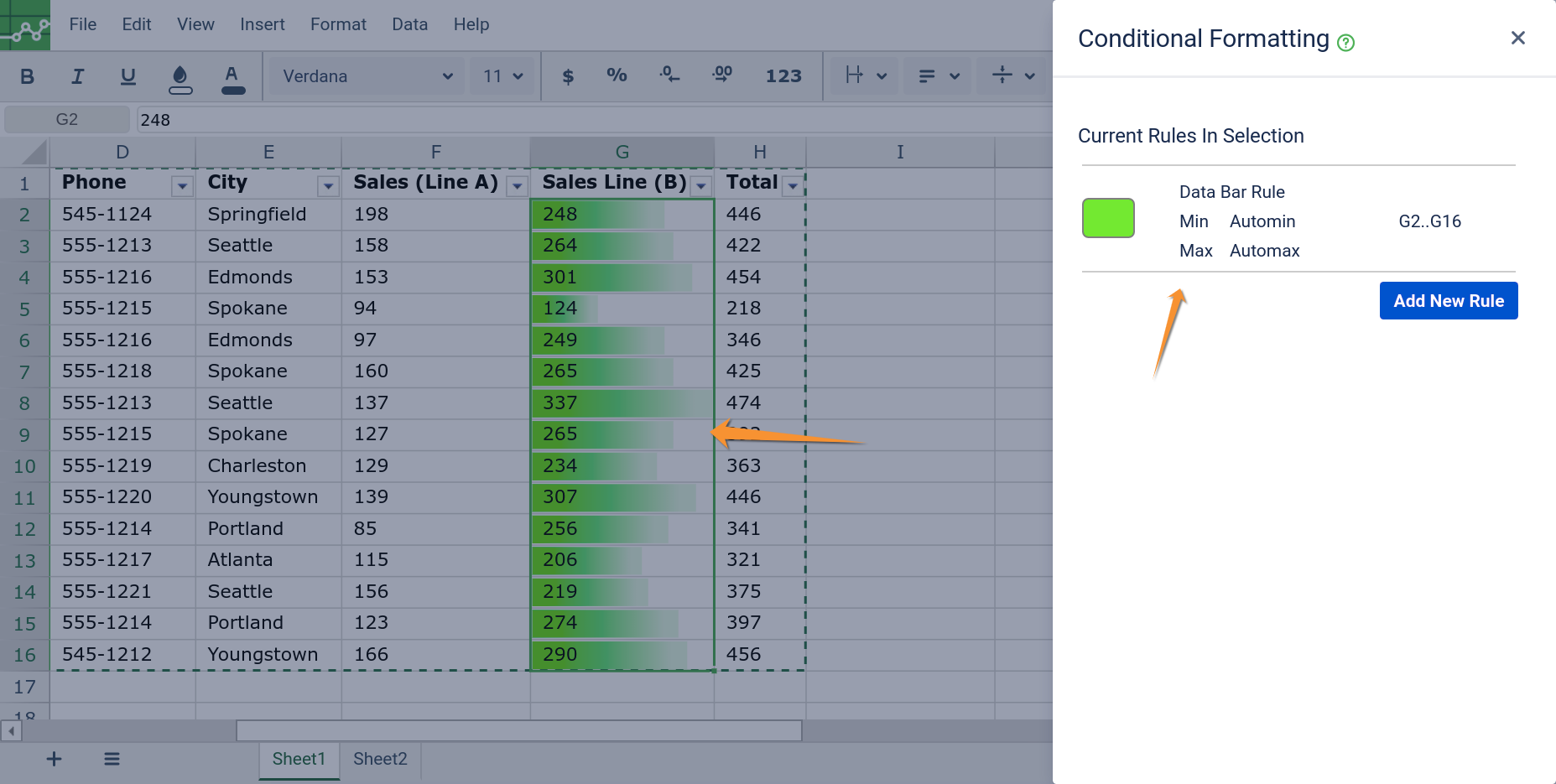
After you have applied all the required rules. Your Excellentable should show the formatting based on the conditions.

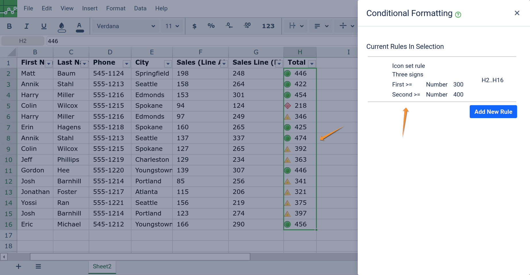
Icon sets will fill appear in the cell along with the
Create a rule by choosing the condition and the style.
In this example we want to highlight the Total with three icons based on values >= 400 as green circle, 400> cell >=300 as yellow triangle and values < 300 as Red squares
In "When" select value "values in icon set rule" and then select "three symbols". Finally select the values under which three signs will appear. Click "Add Rule".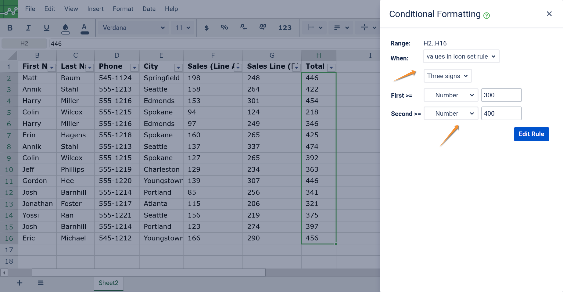
After you have applied all the required rules. Your Excellentable should show the formatting based on the conditions.

Colour scales fill the background of a cell in a gradient scale. Example lowest value can be gradient colour filled to dark red, lower values to red, higher values to green and highest values to dark green
Create a rule by choosing the condition and the style.
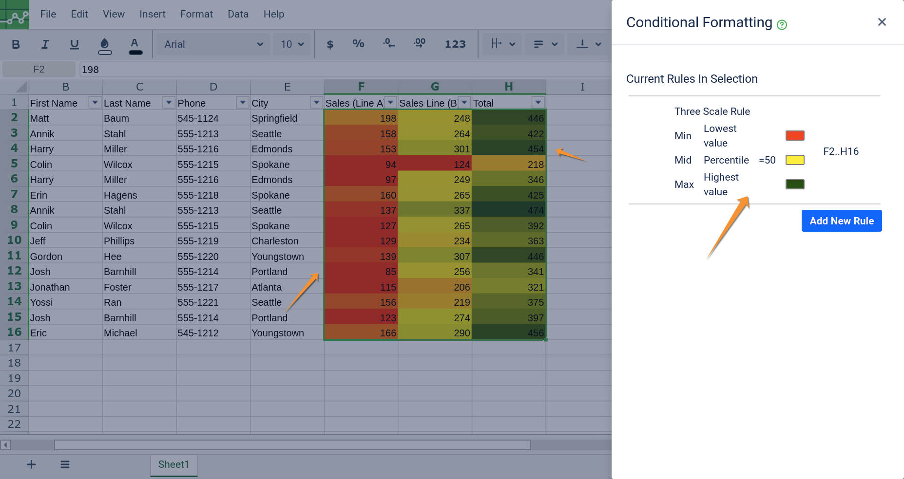
In this example we want to highlight the Total with three colour gradient with lowest values as red, moderate values as yellow, and highest values as green.
In "When" select value "values in three scale rule". In Min select 'lowest value' and select colour red. In the middle values choose percentile 50 and colour yellow and similarly for highest choose the colour green.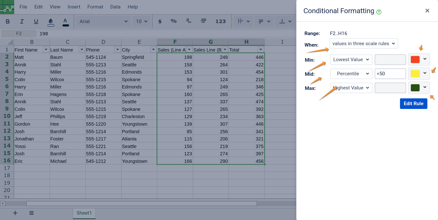
After you have applied all the required rules. Your Excellentable should show the formatting based on the conditions.